Introduction to Neural Networks and Backpropagation

Tue 30 Apr 2024 - 10 min read

The first in a mini-series of blogposts, where I explain concepts in mathematics, statistics and machine learning as a way to get more familiar with the concepts myself.

The Neural Network, also known as a neural net or artificial neural network, is a model of the biological neural networks like that of brains. This model has shown remarkable abilities in many areas of computer science such as image classification, recommendation systems, sequence modelling and other function approximation tasks.

In this little blog post i'll be going over the basics of neural networks as well as a common optimisation algorithm used to train them.

An introduction to Neural Networks

A neural network attempts to model biological nervous systems using many layers of stacks of artificial neurons. The underlying model of these neurons were first popularised by Frank Rosenblatt in 1958 in the paper "The Perceptron: A probabilistic model for information storage and organization in the brain" ¹.

In the brain, neurons receive input signals through dendrites, process these signals in the cell body, and then send an output signal through the axon to connected neurons. Similarly, an artificial neuron in a neural network receives input signals from other neurons, performs a calculation based on these inputs and an activation function, and then sends an output to the next layers of neurons.

Perceptron (single-neuron function)

The perceptron works by receiving $n$ inputs $x$, where every $x$ represents the $i$-th input. These inputs have individually adjustable weights $w$ and together with $b$ make up a linear transformation of the inputs, here a weighted input of $x$ and $w$, and a bias of $b$.

This means multiplying every input $xi$ with the corresponding weight $wi$, and then summing up these weighted transformations and adding the bias. This transformation is denoted by $z$ and makes up the core of our neuron function.

Then the data is passed through to an activation function, a non-linear function that decides whether or not the neuron "activates". Commonly used activation functions include ReLU, sigmoid and hyperbolic tangent, but they all do essentially the same thing. The significance of these activations functions will be quickly explained later.

In the original paper the activation function was a simple stepwise function: $1$ if $z$ was greater than $0$, otherwise $0$.

$$\begin{align} f(x) = \begin{cases} 1 & \text{ if } \sum_{i=1}^{n} w_i x_i + b > 0 \\ 0 & \text{else} \end{cases} \end{align}$$

where

$f(x)$ is the output of the neuron
$xi$ is the $i$-th input
$wi$ is the $i$-th inputs weight
$b$ is the bias
$n$ is the number of inputs

The underlying mathematical model for a neuron uses a more standard notation, where $\sigma$ represents any possible activation function like ReLU.

$$z = \sum_{i=1}^{n} w_i x_i + b > 0$$

$$a = \sigma(z)$$

Where $z$ is a scalar that represents the pre-activation weighted sum and $a$ is a scalar that represents the output of the neuron after the activation.

This becomes cumbersome notation for when we need to describe larger networks with multiple layers or multiple neurons per layer. For this reason we can make use of vector and matrix notation to better organise our data.

Now we can instead represent both $x$ and $w$ as column-vectors.

$$x = \begin{bmatrix} x_{1} \\ x_{2} \\ \vdots \\ x_{n} \end{bmatrix}\hspace{1em} w = \begin{bmatrix} w_{1} \\ w_{2} \\ \vdots \\ w_{n} \\ \end{bmatrix}$$

Here the whole notatoin for the weighted sum can be simplified to the dot-product of the two vectors, where we then add the bias term and it is passed to the activation function.

$$z = w \cdot x + b$$

$$a = \sigma(z)$$

So to summarise, the underlying function of neurons takes an input vector 𝑥 and produces a scalar, which is the dot product of 𝑥 and the weights 𝑤 or the weighted sum of inputs. A bias is added to this, and a nonlinear activation function is applied.

The activation function is important, as the element of a non-linear activation allows a more complex network to model non-linear relationships in data. Without these activations, the network would simply combine linear functions, resulting in an overall linear transformation of the input in the neural network, simplified here:

$$\begin{align} f(x) &= 2x + 1 \\ g(x) &= 3x - 2 \\ f(x) &= g(f(x)) = g(2x + 1) \\ &= 3(2x + 1) - 2 \\ &= 6x + 3 - 2 \\ &= 6x + 1 \end{align}$$

Multiple neurons and the MLP

In a neural network with multiple layers of neurons (multi-layer perceptron), the structure is more complex than a single layer with a single neuron. The term "deep learning" originates from these more complex networks, which consist of multiple layers of neurons.

In a single-layer network with multiple neurons, the output for each individual neuron can be calculated by considering all the previous inputs. This is because the network is densely connected, also known as a fully-connected network or fully-dense network.

In this context, the individually calculated scalars can be represented as a column-vector of the activations in a layer $a^l$, where $l$ denotes the index of the layer.

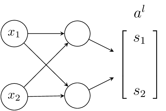
This representation makes it easier to work with multiple layers as it allows us to visualise the interconnection of multiple neurons across the layers.

The weights in the fully-dense layer can now be represented as a matrix $W_{jk}^{l}$ in a layer with $m$ neurons and $n$ inputs, where $l$ is the layer, $j$ is the index of neuron the connection is going to and $k$ is the index of the neuron the connection is coming from.

$$W^{l} = \begin{bmatrix} w^{l}_{11} & w^{l}_{12} & \cdots & w^{l}_{1n} \\ w^{l}_{21} & w^{l}_{22} & \cdots & w^{l}_{2n} \\ \vdots & \vdots & \ddots & \vdots \\ w^{l}_{m1} & w^{l}_{m2} & \cdots & w^{l}_{mn} \end{bmatrix}$$

and the bias can now also be represented as a column-vector of the pre-activation bias terms for every neuron in a layer $l$.

$$b^{l} = \begin{bmatrix} b^{l}_{1}\\ b^{l}_{2}\\ \vdots\\ b^{l}_{m}\\ \end{bmatrix}$$

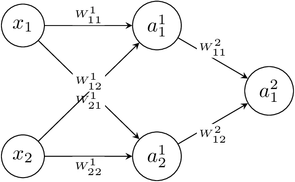
Now the activation for a whole layer $a^l$ based on the activations of the previous layer (inputs) $a^{l-1}$ can be represented as

$$a^l = \sigma(W^{l} \cdot a^{l-1} + b^{l})$$

or more verbously

$$a^l = \sigma\left(\begin{bmatrix} w^{l}_{11} & w^{l}_{12} & \cdots & w^{l}_{1n} \\ w^{l}_{21} & w^{l}_{22} & \cdots & w^{l}_{2n} \\ \vdots & \vdots & \ddots & \vdots \\ w^{l}_{m1} & w^{l}_{m2} & \cdots & w^{l}_{mn} \end{bmatrix} \cdot \begin{bmatrix} a^{l-1}_{1}\\ a^{l-1}_{2}\\ \vdots\\ a^{l-1}_{n} \end{bmatrix} + \begin{bmatrix} b^{l}_{1}\\ b^{l}_{2}\\ \vdots\\ b^{l}_{m} \end{bmatrix}\right)$$

and so the activation of the entire network in the figure above can be represented as

$$a^0 \Rightarrow \sigma(W^1 \cdot a^0 + b^1) = a^1 \Rightarrow \sigma(W^2 \cdot a^1 + b^2) = a^2$$

where $a^0$ are the inputs to the network and $a^2$ is the final output.

This can also be written more generally as

$$\begin{align} a^0 & \Rightarrow \sigma(W^1 \cdot a^0 + b^1) = a^1 \\ & \Rightarrow \sigma(W^2 \cdot a^1 + b^2) = a^2 \Rightarrow \cdots \Rightarrow a^L \end{align}$$

where $a^L$ is the activation in layer $L$ (the amount of layers in the network).

This entire process is called feed-forward and refers to the forward propagation of the inputs through these data transformations until you get an output. Optimising or training these networks is harder but a nice algorithm called Backpropagation makes it easier to grasp.

Backpropagation and optimisation (training)

Neural networks learn by "tuning" these weights based on an error calculation of the network's output with respect to the input. One of the most commonly used methods to achieve this is the backpropagation algorithm.

Backpropagation utilises the chain rule from differential calculus to compute the gradient of the loss function, also known as an objective function, with respect to the weights in the neural network. Backpropagation evaluates how a small change in a weight or bias affects the overall error, and then adjusts these parameters in the direction of minimising the error.

Loss calculation

Typically, a loss function is used to quantify how much the network's predictions deviate from the actual values in the training data. A common choice for the loss function in regression is Mean Squared Error (MSE).

In order to calculate the gradient, the partial derivative of the loss function with respect to the parameters in the network, we use backpropagation and the chain rule.

Let the loss function be $C$ and let $\delta^L$ represent the loss in the last layer $L$. Here the loss is defined as $\frac{\partial{C}}{\partial{z^l}}$ as we want to understand how the pre-activations in a layer $l$ ($z^l$) affect $C$.

We start by using the chain rule, $\frac{\partial{y}}{\partial{x}} = \frac{\partial{y}}{\partial{u}} \frac{\partial{u}}{\partial{x}}$, in order to calculate the loss in the last layer $L$.

$$\begin{align} \delta^L &= \frac{\partial{C}}{\partial{a^L}} \frac{\partial{a^L}}{\partial{z^L}} \\ &= \frac{\partial{C}}{\partial{a^L}} \odot \sigma'(z^L) \end{align}$$

In order to calculate the loss in any layer $l$ ($\delta^l$) we start from the loss function and calculate $\frac{\partial{C}}{\partial{z^l}}$ backwards from $C$ to the layer $l$.

We can use the chain rule to compute the loss in the last layer $L$ as well as step-by-step backwards from the last layer $L$ to layer $l$:

$$\begin{align} & \frac{\partial C}{\partial z^L} \\ & \frac{\partial C}{\partial a^L} \cdot \frac{\partial a^L}{\partial z^L} \\ & \frac{\partial C}{\partial a^{L-1}} \cdot \frac{\partial a^{L-1}}{\partial z^{L-1}} \cdot \frac{\partial z^{L-1}}{\partial a^{L-2}} \cdot \ldots \cdot \frac{\partial a^l}{\partial z^l} \\ \end{align}$$

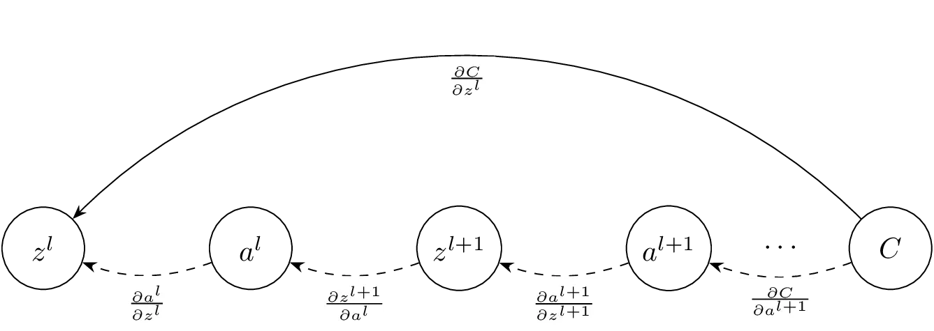
Deriving from this method we can more neatly represent the loss in a layer $l$ by looking at the next layer $l+1$ and represent $\frac{\partial{C}}{\partial{z^{l}}}$ as

$$\frac{\partial{C}}{\partial{z^l}} = \frac{\partial{a^l}}{\partial{z^l}} \cdot \frac{\partial{z^{l+1}}}{\partial{a^l}} \cdot \frac{\partial{C}}{\partial{z^{l+1}}}$$

whose components are

$\frac{\partial{a^l}}{\partial{z^l}}$ which is the partial derivative of the activation function $\sigma$ applied to $z^l$, $\sigma'(z^l)$.

$\frac{\partial{z^{l+1}}}{\partial{a^l}}$ which is the partial derivative of the pre-activation in the next layer $W^{l+1} \cdot a^l + b^{l+1}$ with respect to $a^l$. Here, the partial derivative of $z^{l+1}$ with respect to $a^l$ is $(W^{l+1})^\intercal$ (transposed), as the partial derivative of a matrix product $AB$ with respect to $B$ is $A^\intercal$. This also makes intuitive sense since we transpose the matrix to propagate the loss backwards through the network.

$\frac{\partial{C}}{\partial{z^{l+1}}}$ which is the partial derivative of the loss function $C$ with respect to the pre-activations $z^{l+1}$ in the next layer, which can also be rewritten as $\delta^{l+1}$.

Now, we can compute the loss $\delta^l$ in any layer $l$:

$$\delta^l = \frac{\partial{C}}{\partial{z^l}} = \frac{\partial{a^l}}{\partial{z^l}} \cdot \frac{\partial{z^{l+1}}}{\partial{a^l}} \cdot \frac{\partial{C}}{\partial{z^{l+1}}}$$

Substituting the previously found components, we get:

$$\delta^l = \sigma'(z^l) \odot ((W^{l+1})^\intercal \delta^{l+1})$$

Finally, the gradients are computed, which are the changes in the loss function $C$ with respect to the parameters $W^l$ and $b^l$:

$$\begin{align} \frac{\partial C}{\partial W^l} &= \frac{\partial z^l}{\partial W^l} \frac{\partial C}{\partial z^l} \\ &= a^{l-1} \cdot \frac{\partial C}{\partial z^l} \\ &= \frac{\partial C}{\partial z^l} \cdot a^{l-1} \\ \end{align}$$

$$\begin{align} \frac{\partial C}{\partial b^l} &= \frac{\partial z^l}{\partial b^l} \frac{\partial C}{\partial z^l} \\ &= 1 \cdot \frac{\partial C}{\partial z^l} \\ &= \delta^l \\ \end{align}$$

Now that we know how each parameter in our neural net influences the loss, we just need to figure out how to optimise our network to minimise the loss. Luckily, there is a simple and effective way of doing that as we've already done the hard part.

Gradient descent and optimisation

The gradients we calculated are used in optimisation algorithms to adjust randomly initialised parameters, the weights and biases, in a neural network with the aim of minimising the loss function.

Stochastic gradient descent (SGD) is a variant of gradient descent used in machine learning. SGD updates the weights iteratively for each training instance based on the gradient of the error function, which is more efficient for large datasets.

$$\theta = \theta - \eta \cdot \nabla C(\theta)$$

where $\theta$ is the parameters, $\eta$ is the learning rate that controls the size of the update, and $\nabla C(\theta)$ ($\frac{\partial{C}}{\partial{\theta}}$) is the gradient of the error function with respect to the parameters $\theta$.

In this way, a network can iteratively learn to minimise the loss for an arbitrary underlying function.

1. Rosenblatt, F. 1958. “The perceptron: A probabilistic model for information storage and organization in the brain”. Psychological Review 65 (6): 386–408. https://doi.org/10.1037/h0042519. ↩